
Hacker
Professional
- Messages
- 1,041
- Reaction score
- 857
- Points
- 113
The content of the article
For each example, I'll provide Python 3.7 code. You can run it and see how it all works. To run the examples, you need the Tensorflow library. You can install it with the command pip install tensorflow-gpuif the video card supports CUDA, otherwise use the command pip install tensorflow. Computing with CUDA is several times faster, so if your video card supports it, it will save a lot of time. And don't forget to install the network training datasets by the team pip install tensorflow-datasets.
How a neural network works
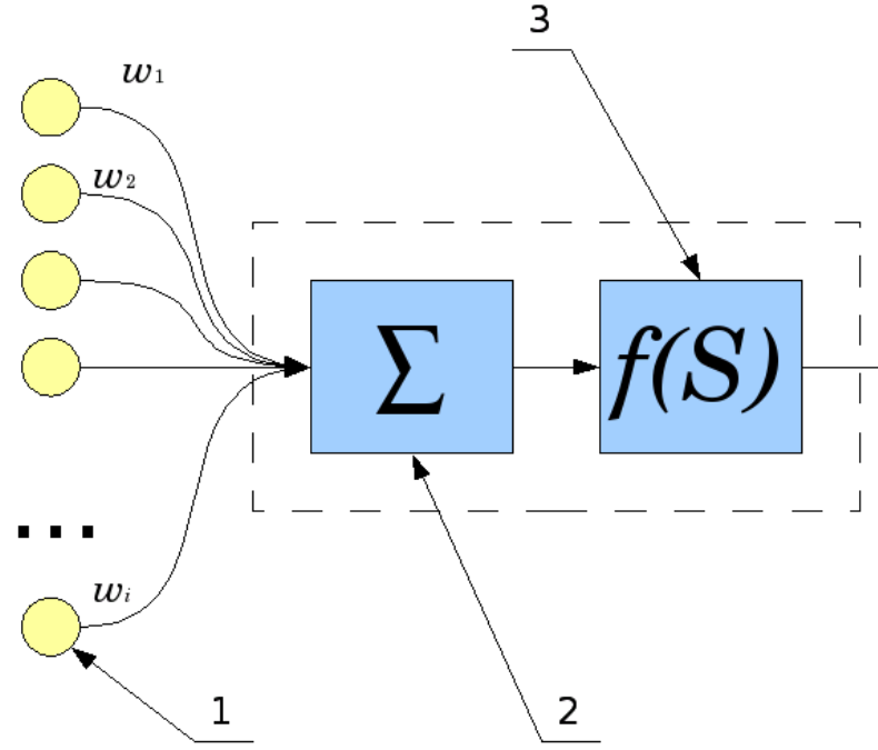
How does one neuron work? Signals from inputs (1) are summed (2), and each input has its own "gain" - w. Then the “activation function” (3) is applied to the resulting result.
The types of this function are different, it can be:
Let's consider the simplest neural network and teach it to perform a function XOR. Of course, calculating XOR with a neural network has no practical sense. But it is it that will help us understand the basic principles of learning and using a neural network and will allow us to follow its work step by step. This would be too complicated and cumbersome with networks of larger dimensions.
The simplest neural network
First you need to connect the necessary libraries, in our case it is tensorflow. I also turn off debug output and work with the GPU, they are not useful to us. To work with arrays, we need a library numpy.
We are now ready to create a neural network. Thanks to Tensorflow, it only takes four lines of code.
We created a neural network model - a class Sequential- and added two layers to it: input and output. Such a network is called a multilayer perceptron, and in general it looks like this.
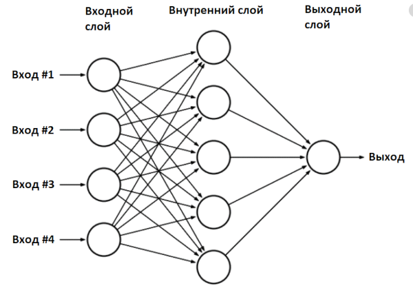
In our case, the network has two inputs (outer layer), two neurons in the inner layer and one output.
You can see what we got:
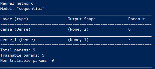
Training a neural network consists in finding the values of the parameters of this network.
Our network has nine parameters. To train it, we need an initial dataset, in our case, these are the results of the function XOR.
The function fitstarts the learning algorithm, which we will run a thousand times, at each iteration the network parameters will be adjusted. Our network is small, so learning will be quick. After training, the network can already be used:
The result is consistent with what the network has learned.
Network test:
We can display all the values of the found coefficients on the screen.
Result:
The internal implementation of the function model.predict_probalooks like this:
Consider the situation when the values [0,1] were fed to the network input:
An activation function ReLu(rectified linear unit) is simply replacing negative elements with zero.
Now the found values fall on the second layer.
Finally, as an output, a function is used Sigmoidthat converts the values to the range 0 ... 1:
We made the usual operations of addition and multiplication of matrices, and received the answer: XOR(0,1) = 1.
I advise you to experiment with this Python example yourself. For example, you can change the number of neurons in the inner layer. Two neurons, as in our case, is the very minimum for the network to work.
But the learning algorithm used in Keras is not perfect: neural networks cannot always learn in 1000 iterations, and the results are not always correct. For example, Keras initializes the initial values with random values, and the result may differ each time it is run. My network with two neurons trained successfully only 20% of the time. An abnormal network operation looks something like this:
But that's okay. If you see that the neural network does not produce the correct results during training, the training algorithm can be run again. A properly trained network can then be used without restrictions.
You can make the network smarter: use four neurons instead of two, for this you just need to replace a line of code model.add(Dense(2, input_dim=2, activation='relu'))with model.add(Dense(4, input_dim=2, activation='relu')). Such a network is trained already in 60% of cases, a network of six neurons is trained the first time with a 90% probability.
All parameters of the neural network are completely determined by the coefficients. Having trained the network, you can write the network parameters to disk, and then use the already prepared trained network. We will actively use this.
Digit recognition - MLP network
Let's consider a practical task, quite classical for neural networks, - digit recognition. To do this, we will take the multilayer perceptron network already known to us, the same one that we used for the function XOR. The input data will be images of 28 × 28 pixels. This size was chosen because there is already a ready-made base of handwritten numbers MNIST, which is stored in exactly this format.
For convenience, let's split the code into several functions. The first part is creating the model.
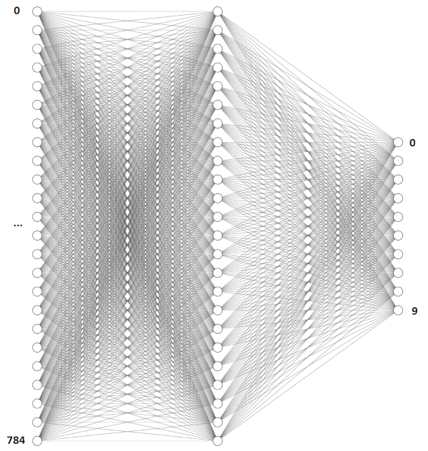
image_w*image_hValues will be fed to the network input - in our case it is 28 × 28 = 784. The number of neurons in the inner layer is the same and equal to 784.
There is one peculiarity with the recognition of numbers. As we saw in the previous example, the output of the neural network can lie in the range 0 ... 1, but we need to recognize the numbers from 0 to 9. What to do? To recognize numbers, we create a network with ten outputs, and one will be at the output corresponding to the desired digit.
The structure of a single neuron is so simple that it doesn't even need a computer to use it. Recently, scientists were able to implement a neural network similar to ours, in the form of a piece of glass - such a network does not require power and does not contain a single electronic component inside.
When the neural network is created, it needs to be trained. First, you need to load the MNIST dataset and convert the data to the desired format.
We have two data blocks: trainand test- one is used for training, the second is for verifying the results. This is a common practice, it is desirable to train and test a neural network on different datasets.
Ready network learning code:
We create a model, train it and write the result to a file.
On my computer with a Core i7 and a GeForce 1060 video card, the process takes 18 seconds and 50 seconds with calculations without a GPU - almost three times longer. So, if you want to experiment with neural networks, a good graphics card is highly desirable.
Now let's write a function for recognizing a picture from a file - that's what this network was created for. For recognition, we have to bring the picture to the same format - a black and white image of 28 x 28 pixels.
Now using a neural network is pretty simple. I created five images with different numbers in Paint and ran the code.
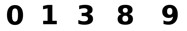
The result, alas, is not ideal: 0, 1, 3, 6 and 6. The neural network successfully recognized 0, 1, and 3, but confused 8 and 9 with the number 6. Of course, you can change the number of neurons, the number of training iterations. In addition, these numbers were not handwritten, so no one promised us a 100% result.
Such a neural network with an additional layer and a large number of neurons correctly recognizes the number eight, but still confuses 8 and 9.
If you want, you can train the neural network on your dataset, but this requires quite a lot of data (MNIST contains 60 thousand sample numbers). Those interested can experiment on their own, and we will go further and consider convolutional networks (CNN, Convolutional Neural Network), which are more efficient for image recognition.
Digit Recognition - Convolutional Network (CNN)
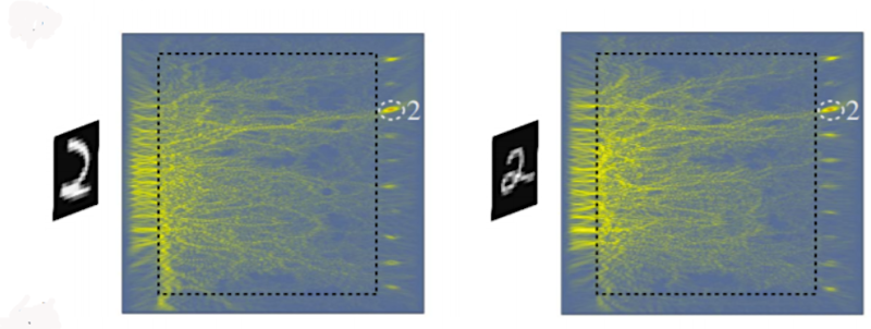
In the previous example, we used a 28x28 image as a simple one-dimensional array of 784 digits. This approach, in principle, works, but starts to malfunction if the image is shifted, for example. It is enough in the previous example to shift the digit to the corner of the picture, and the program will no longer recognize it.
Convolutional networks are much more efficient in this regard - they use the principle of convolution, according to which the so-called kernel (kernel) moves along the image and highlights the key effects in the picture, if any. Then the obtained result is reported to the "normal" neural network, which produces the finished result.
The layer Conv2Dis responsible for convolution of the input image with a 3 × 3 kernel, and the layer MaxPooling2Dperforms downsampling - reduction of the image size. At the output of the network, we see the layer already familiar to us Dense, which we used earlier.
As in the previous case, the network must first be trained, and the principle is the same, except that we are working with two-dimensional images.
All is ready. We create a model, train it and write the model to a file:
Training a neural network with the same MNIST database of 60 thousand images takes 46 seconds using Nvidia CUDA and about five minutes without it.
Now we can use the neural network for image recognition:
The result is much more accurate, as expected: [0, 1, 3, 8, 9].
All is ready! Now you have a program that can recognize numbers. With Python, your code will run anywhere - on Windows and Linux operating systems. You can even run it on a Raspberry Pi if you want.
You probably want to know if letters can be recognized in the same way? Yes, you just have to increase the number of network outputs and find a suitable set of pictures for training.
Hope you have enough information to experiment with. In addition, it is much easier to deal with a real example before your eyes!
- How a neural network works
- The simplest neural network
- Digit recognition - MLP network
- Digit Recognition - Convolutional Network (CNN)
For each example, I'll provide Python 3.7 code. You can run it and see how it all works. To run the examples, you need the Tensorflow library. You can install it with the command pip install tensorflow-gpuif the video card supports CUDA, otherwise use the command pip install tensorflow. Computing with CUDA is several times faster, so if your video card supports it, it will save a lot of time. And don't forget to install the network training datasets by the team pip install tensorflow-datasets.
How a neural network works
How does one neuron work? Signals from inputs (1) are summed (2), and each input has its own "gain" - w. Then the “activation function” (3) is applied to the resulting result.
The types of this function are different, it can be:
- rectangular (output 0 or 1);
- linear;
- in the form of a sigmoid.
Let's consider the simplest neural network and teach it to perform a function XOR. Of course, calculating XOR with a neural network has no practical sense. But it is it that will help us understand the basic principles of learning and using a neural network and will allow us to follow its work step by step. This would be too complicated and cumbersome with networks of larger dimensions.
The simplest neural network
First you need to connect the necessary libraries, in our case it is tensorflow. I also turn off debug output and work with the GPU, they are not useful to us. To work with arrays, we need a library numpy.
Code:
import
os.environ['TF_CPP_MIN_LOG_LEVEL'] = '3'
os.environ["CUDA_VISIBLE_DEVICES"] = "-1"

from tensorflow import keras
from tensorflow.keras import layers
from tensorflow.keras import Sequential
from tensorflow.keras.layers import Conv2D, MaxPooling2D, Flatten, Dense, Dropout, Activation, BatchNormalization, AveragePooling2D
from tensorflow.keras.optimizers import SGD, RMSprop, Adam
import tensorflow_datasets as tfds  # pip install tensorflow-datasets
import tensorflow as tf
import logging
import numpy as np

tf.logging.set_verbosity(tf.logging.ERROR)
tf.get_logger().setLevel(logging.ERROR)
We are now ready to create a neural network. Thanks to Tensorflow, it only takes four lines of code.
Code:
model = Sequential()
model.add(Dense(2, input_dim=2, activation='relu'))
model.add(Dense(1, activation='sigmoid'))
model.compile(loss='binary_crossentropy', optimizer=SGD(lr=0.1))
We created a neural network model - a class Sequential- and added two layers to it: input and output. Such a network is called a multilayer perceptron, and in general it looks like this.
In our case, the network has two inputs (outer layer), two neurons in the inner layer and one output.
You can see what we got:
Code:
print(model.summary())Training a neural network consists in finding the values of the parameters of this network.
Our network has nine parameters. To train it, we need an initial dataset, in our case, these are the results of the function XOR.
Code:
X = np.array([[0,0], [0,1], [1,0], [1,1]])
y = np.array ([[0], [1], [1], [0]])
model.fit(X, y, batch_size=1, epochs=1000, verbose=0)
The function fitstarts the learning algorithm, which we will run a thousand times, at each iteration the network parameters will be adjusted. Our network is small, so learning will be quick. After training, the network can already be used:
Code:
print("Network test:")
print("XOR(0,0):", model.predict_proba(np.array([[0, 0]])))
print("XOR(0,1):", model.predict_proba(np.array([[0, 1]])))
print("XOR(1,0):", model.predict_proba(np.array([[1, 0]])))
print("XOR(1,1):", model.predict_proba(np.array([[1, 1]])))
The result is consistent with what the network has learned.
Network test:
Code:
XOR (0.0): [[0.00741202]]
XOR (0.1): [[0.99845064]]
XOR (1.0): [[0.9984376]]
XOR (1,1): [[0.00741202]]
We can display all the values of the found coefficients on the screen.
Code:
## Parameters layer 1
W1 = model.get_weights()[0]
b1 = model.get_weights()[1]
## Parameters layer 2
W2 = model.get_weights()[2]
b2 = model.get_weights()[3]

print("W1:", W1)
print("b1:", b1)
print("W2:", W2)
print("b2:", b2)
print()
Result:
Code:
W1: [[ 2.8668058 -2.904025 ] [-2.871452 2.9036295]]
b1: [-0.00128211 -0.00191825]
W2: [[3.9633768] [3.9168582]]
b2: [-4.897212]
The internal implementation of the function model.predict_probalooks like this:
Code:
x_in = [0, 1]
## Input
X1 = np.array([x_in], "float32")
## First layer calculation
L1 = e.g. dot (X1, W1) + b1
## Relu activation function: y = max(0, x)
X2 = e.g. maximum (L1, 0)
## Second layer calculation
L2 = np.dot(X2, W2) + b2
## Sigmoid
output = 1 / (1 + np.exp(-L2))
Consider the situation when the values [0,1] were fed to the network input:
Code:
L1 = X1W1 + b1 = [02.8668058 + 1-2.871452 + -0.0012821, 0-2.904025 + 1*2.9036295 + -0.00191825] = [-2.8727343 2.9017112]An activation function ReLu(rectified linear unit) is simply replacing negative elements with zero.
Code:
X2 = e.g. maximum (L1, 0) = [0. 2.9017112]Now the found values fall on the second layer.
Code:
L2 = X2 W2 + b2 = 0 3.9633768 + 2.9017112 * 3.9633768 + -4.897212 = 6.468379Finally, as an output, a function is used Sigmoidthat converts the values to the range 0 ... 1:
Code:
output = 1 / (1 + np.exp(-L2)) = 0.99845064We made the usual operations of addition and multiplication of matrices, and received the answer: XOR(0,1) = 1.
I advise you to experiment with this Python example yourself. For example, you can change the number of neurons in the inner layer. Two neurons, as in our case, is the very minimum for the network to work.
But the learning algorithm used in Keras is not perfect: neural networks cannot always learn in 1000 iterations, and the results are not always correct. For example, Keras initializes the initial values with random values, and the result may differ each time it is run. My network with two neurons trained successfully only 20% of the time. An abnormal network operation looks something like this:
Code:
XOR (0.0): [[0.66549516]]
XOR (0.1): [[0.66549516]]
XOR (1.0): [[0.66549516]]
XOR (1,1): [[0.00174837]]
But that's okay. If you see that the neural network does not produce the correct results during training, the training algorithm can be run again. A properly trained network can then be used without restrictions.
You can make the network smarter: use four neurons instead of two, for this you just need to replace a line of code model.add(Dense(2, input_dim=2, activation='relu'))with model.add(Dense(4, input_dim=2, activation='relu')). Such a network is trained already in 60% of cases, a network of six neurons is trained the first time with a 90% probability.
All parameters of the neural network are completely determined by the coefficients. Having trained the network, you can write the network parameters to disk, and then use the already prepared trained network. We will actively use this.
Digit recognition - MLP network
Let's consider a practical task, quite classical for neural networks, - digit recognition. To do this, we will take the multilayer perceptron network already known to us, the same one that we used for the function XOR. The input data will be images of 28 × 28 pixels. This size was chosen because there is already a ready-made base of handwritten numbers MNIST, which is stored in exactly this format.
For convenience, let's split the code into several functions. The first part is creating the model.
Code:
def mnist_make_model(image_w: int, image_h: int):
   # Neural network model
   model = Sequential()
   model.add(Dense(784, activation='relu', input_shape=(image_w*image_h,)))
   model.add(Dense(10, activation='softmax'))
   model.compile(loss='categorical_crossentropy', optimizer=RMSprop(), metrics=['accuracy'])
   return model
image_w*image_hValues will be fed to the network input - in our case it is 28 × 28 = 784. The number of neurons in the inner layer is the same and equal to 784.
There is one peculiarity with the recognition of numbers. As we saw in the previous example, the output of the neural network can lie in the range 0 ... 1, but we need to recognize the numbers from 0 to 9. What to do? To recognize numbers, we create a network with ten outputs, and one will be at the output corresponding to the desired digit.
The structure of a single neuron is so simple that it doesn't even need a computer to use it. Recently, scientists were able to implement a neural network similar to ours, in the form of a piece of glass - such a network does not require power and does not contain a single electronic component inside.
When the neural network is created, it needs to be trained. First, you need to load the MNIST dataset and convert the data to the desired format.
We have two data blocks: trainand test- one is used for training, the second is for verifying the results. This is a common practice, it is desirable to train and test a neural network on different datasets.
Code:
def mnist_mlp_train(model):
(x_train, y_train), (x_test, y_test) = keras.datasets.mnist.load_data()
# x_train: 60000x28x28 array, x_test: 10000x28x28 array
image_size = x_train.shape[1]
train_data = x_train.reshape(x_train.shape[0], image_size*image_size)
test_data = x_test.reshape(x_test.shape[0], image_size*image_size)
train_data = train_data.astype('float32')
test_data = test_data.astype('float32')
train_data /= 255.0
test_data /= 255.0
# encode the labels - we have 10 output classes
# 3 -> [0 0 0 1 0 0 0 0 0 0], 5 -> [0 0 0 0 0 1 0 0 0 0]
num_classes = 10
train_labels_cat = keras.utils.to_categorical(y_train, num_classes)
test_labels_cat = keras.utils.to_categorical(y_test, num_classes)
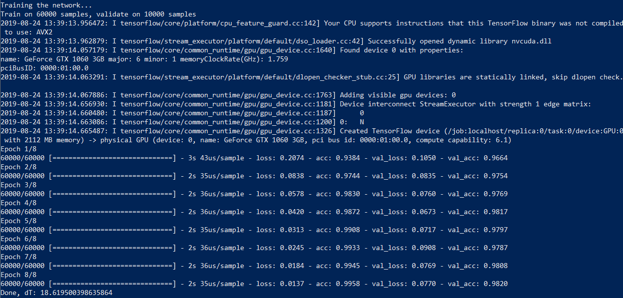
print("Training the network...")
t_start = time.time()
# Start training the network
model.fit(train_data, train_labels_cat, epochs=8, batch_size=64,
verbose=1, validation_data=(test_data, test_labels_cat))Ready network learning code:
Code:
model = mnist_make_model(image_w=28, image_h=28)
mnist_mlp_train (model)
model.save('mlp_digits_28x28.h5')
We create a model, train it and write the result to a file.
On my computer with a Core i7 and a GeForce 1060 video card, the process takes 18 seconds and 50 seconds with calculations without a GPU - almost three times longer. So, if you want to experiment with neural networks, a good graphics card is highly desirable.
Now let's write a function for recognizing a picture from a file - that's what this network was created for. For recognition, we have to bring the picture to the same format - a black and white image of 28 x 28 pixels.
Code:
def mlp_digits_predict(model, image_file):
   image_size = 28
   img = keras.preprocessing.image.load_img(image_file, target_size=(image_size, image_size), color_mode='grayscale')
   img_arr = np.expand_dims(img, axis=0)
   img_arr = 1 - img_arr/255.0
   img_arr = img_arr.reshape((1, image_size*image_size))

   result = model.predict_classes([img_arr])
   return result[0]
Now using a neural network is pretty simple. I created five images with different numbers in Paint and ran the code.
Code:
model = tf.keras.models.load_model('mlp_digits_28x28.h5')
print(mlp_digits_predict(model, 'digit_0.png'))
print(mlp_digits_predict(model, 'digit_1.png'))
print(mlp_digits_predict(model, 'digit_3.png'))
print(mlp_digits_predict(model, 'digit_8.png'))
print(mlp_digits_predict(model, 'digit_9.png'))
The result, alas, is not ideal: 0, 1, 3, 6 and 6. The neural network successfully recognized 0, 1, and 3, but confused 8 and 9 with the number 6. Of course, you can change the number of neurons, the number of training iterations. In addition, these numbers were not handwritten, so no one promised us a 100% result.
Such a neural network with an additional layer and a large number of neurons correctly recognizes the number eight, but still confuses 8 and 9.
Code:
def mnist_make_model2(image_w: int, image_h: int):
   # Neural network model
   model = Sequential()
   model.add(Dense(1024, activation='relu', input_shape=(image_w*image_h,)))
   model.add(Dropout(0.2))  # rate 0.2 - set 20% of inputs to zero
   model.add(Dense(1024, activation='relu'))
   model.add(Dropout(0.2))
   model.add(Dense(10, activation='softmax'))
   model.compile(loss='categorical_crossentropy', optimizer=RMSprop(),
            metrics=['accuracy'])
   return model
If you want, you can train the neural network on your dataset, but this requires quite a lot of data (MNIST contains 60 thousand sample numbers). Those interested can experiment on their own, and we will go further and consider convolutional networks (CNN, Convolutional Neural Network), which are more efficient for image recognition.
Digit Recognition - Convolutional Network (CNN)
In the previous example, we used a 28x28 image as a simple one-dimensional array of 784 digits. This approach, in principle, works, but starts to malfunction if the image is shifted, for example. It is enough in the previous example to shift the digit to the corner of the picture, and the program will no longer recognize it.
Convolutional networks are much more efficient in this regard - they use the principle of convolution, according to which the so-called kernel (kernel) moves along the image and highlights the key effects in the picture, if any. Then the obtained result is reported to the "normal" neural network, which produces the finished result.
Code:
def mnist_cnn_model():
   image_size = 28
   num_channels = 1  # 1 for grayscale images
   num_classes = 10  # Number of outputs
   model = Sequential()
   model.add(Conv2D(filters=32, kernel_size=(3,3), activation='relu',
            padding='same',
input_shape=(image_size, image_size, num_channels)))
   model.add(MaxPooling2D(pool_size=(2, 2)))
   model.add(Conv2D(filters=64, kernel_size=(3, 3), activation='relu',
            padding='same'))
   model.add(MaxPooling2D(pool_size=(2, 2)))
   model.add(Conv2D(filters=64, kernel_size=(3, 3), activation='relu',
            padding='same'))
   model.add(MaxPooling2D(pool_size=(2, 2)))
   model.add(Flatten())
   # Densely connected layers
   model.add(Dense(128, activation='relu'))
   # Output layer
   model.add(Dense(num_classes, activation='softmax'))
   model.compile(optimizer=Adam(), loss='categorical_crossentropy',
            metrics=['accuracy'])
   return model
The layer Conv2Dis responsible for convolution of the input image with a 3 × 3 kernel, and the layer MaxPooling2Dperforms downsampling - reduction of the image size. At the output of the network, we see the layer already familiar to us Dense, which we used earlier.
As in the previous case, the network must first be trained, and the principle is the same, except that we are working with two-dimensional images.
Code:
def mnist_cnn_train(model):
   (train_digits, train_labels), (test_digits, test_labels) = keras.datasets.mnist.load_data()

   # Get image size
   image_size = 28
   num_channels = 1  # 1 for grayscale images

   # re-shape and re-scale the images data
   train_data = np.reshape(train_digits, (train_digits.shape[0], image_size, image_size, num_channels))
   train_data = train_data.astype('float32') / 255.0
   # encode the labels - we have 10 output classes
   # 3 -> [0 0 0 1 0 0 0 0 0 0], 5 -> [0 0 0 0 0 1 0 0 0 0]
   num_classes = 10
   train_labels_cat = keras.utils.to_categorical(train_labels, num_classes)

   # re-shape and re-scale the images validation data
   val_data = np.reshape(test_digits, (test_digits.shape[0], image_size, image_size, num_channels))
   val_data = val_data.astype('float32') / 255.0
   # encode the labels - we have 10 output classes
   val_labels_cat = keras.utils.to_categorical(test_labels, num_classes)

   print("Training the network...")
   t_start = time.time()

   # Start training the network
   model.fit(train_data, train_labels_cat, epochs=8, batch_size=64,
        validation_data=(val_data, val_labels_cat))

   print("Done, dT:", time.time() - t_start)

   return model
All is ready. We create a model, train it and write the model to a file:
Code:
model = mnist_cnn_model()
mnist_cnn_train(model)
model.save('cnn_digits_28x28.h5')
Training a neural network with the same MNIST database of 60 thousand images takes 46 seconds using Nvidia CUDA and about five minutes without it.
Now we can use the neural network for image recognition:
Code:
def cnn_digits_predict(model, image_file):
   image_size = 28
   img = keras.preprocessing.image.load_img(image_file,
target_size=(image_size, image_size), color_mode='grayscale')
   img_arr = np.expand_dims(img, axis=0)
   img_arr = 1 - img_arr/255.0
   img_arr = img_arr.reshape((1, 28, 28, 1))

   result = model.predict_classes([img_arr])
   return result[0]

model = tf.keras.models.load_model('cnn_digits_28x28.h5')
print(cnn_digits_predict(model, 'digit_0.png'))
print(cnn_digits_predict(model, 'digit_1.png'))
print(cnn_digits_predict(model, 'digit_3.png'))
print(cnn_digits_predict(model, 'digit_8.png'))
print(cnn_digits_predict(model, 'digit_9.png'))
The result is much more accurate, as expected: [0, 1, 3, 8, 9].
All is ready! Now you have a program that can recognize numbers. With Python, your code will run anywhere - on Windows and Linux operating systems. You can even run it on a Raspberry Pi if you want.
You probably want to know if letters can be recognized in the same way? Yes, you just have to increase the number of network outputs and find a suitable set of pictures for training.
Hope you have enough information to experiment with. In addition, it is much easier to deal with a real example before your eyes!